Workshop 2.1: R Demo Notebook

Workshop 2.1: R Demo Notebook#

Contributors:
- Ashwin Patil (@ashwinpatil)
- Jose Rodriguez (@Cyb3rPandah)
- Ian Hellen (@ianhellen)
Agenda:
- Jupyter is not just Python
Notebook: https://aka.ms/Jupyterthon-ws-2-1
License: Creative Commons Attribution-ShareAlike 4.0 International
Q&A - OTR Discord #Jupyterthon #WORKSHOP DAY 2 - JUPYTER ADVANCED

Anomaly detection and threat hunting on Windows logon data using anomalize#

Reference original blog post by Russ Mcree:

https://holisticinfosec.blogspot.com/2018/06/toolsmith-133-anomaly-detection-threat.html

#Suppress R Warnings
options(warn=-1)
# Load R Packages
pkgs <- c(pkgs <- c("tibbletime", "tidyverse","anomalize", "jsonlite", "curl", "httr", "lubridate","dplyr"))
sapply(pkgs, function(x) suppressPackageStartupMessages(require(x, character.only = T)))

tibbletime: TRUE
tidyverse: TRUE
anomalize: TRUE
jsonlite: TRUE
curl: TRUE
httr: TRUE
lubridate: TRUE
dplyr: TRUE

Install Missing packages#

install.packages("tibbletime")

Updating HTML index of packages in '.Library'

Making 'packages.html' ...
 done

install.packages("anomalize")

Updating HTML index of packages in '.Library'

Making 'packages.html' ...
 done

#Suppress R Warnings
options(warn=-1)
# Load R Packages
pkgs <- c(pkgs <- c("tibbletime", "tidyverse","anomalize", "jsonlite", "curl", "httr", "lubridate","dplyr"))
sapply(pkgs, function(x) suppressPackageStartupMessages(require(x, character.only = T)))

tibbletime: TRUE
tidyverse: TRUE
anomalize: TRUE
jsonlite: TRUE
curl: TRUE
httr: TRUE
lubridate: TRUE
dplyr: TRUE

Read csv using R#

# Read CSV into R
urlfile<-'https://raw.githubusercontent.com/ashwin-patil/threat-hunting-with-notebooks/master/rawdata/UserLogons-demo.csv'
userlogondemo<-read.csv(urlfile)

Printing the structure of the data#

str(userlogondemo)

'data.frame':	2844 obs. of  6 variables:
 $ Date           : chr  "1/3/2018" "1/3/2018" "1/3/2018" "1/3/2018" ...
 $ EventId        : chr  "Microsoft-Windows-Security-Auditing:4624" "Microsoft-Windows-Security-Auditing:4624" "Microsoft-Windows-Security-Auditing:4624" "Microsoft-Windows-Security-Auditing:4624" ...
 $ AccountNtDomain: chr  "LABDOMAIN.LOCAL" "LABDOMAIN.LOCAL" "LABDOMAIN.LOCAL" "LABDOMAIN.LOCAL" ...
 $ AccountName    : chr  "SRVACCNT-01" "SRVACCNT-01" "SRVACCNT-01" "SRVACCNT-01" ...
 $ logontype      : int  10 11 2 4 7 10 4 3 3 5 ...
 $ TotalLogons    : int  28 2 15592 259 9 1 23 65 7 60 ...

Printing Sample Rows from the dataset#

head(userlogondemo)

A data.frame: 6 × 6
	Date	EventId	AccountNtDomain	AccountName	logontype	TotalLogons
	<chr>	<chr>	<chr>	<chr>	<int>	<int>
1	1/3/2018	Microsoft-Windows-Security-Auditing:4624	LABDOMAIN.LOCAL	SRVACCNT-01	10	28
2	1/3/2018	Microsoft-Windows-Security-Auditing:4624	LABDOMAIN.LOCAL	SRVACCNT-01	11	2
3	1/3/2018	Microsoft-Windows-Security-Auditing:4624	LABDOMAIN.LOCAL	SRVACCNT-01	2	15592
4	1/3/2018	Microsoft-Windows-Security-Auditing:4624	LABDOMAIN.LOCAL	SRVACCNT-01	4	259
5	1/3/2018	Microsoft-Windows-Security-Auditing:4624	LABDOMAIN.LOCAL	SRVACCNT-01	7	9
6	1/3/2018	Microsoft-Windows-Security-Auditing:4624	LABDOMAIN.LOCAL	SRVACCNT-01	10	1

#Read Downloaded csv and arrange by columns
userlogonsummary <- userlogondemo %>%
                    arrange(AccountName,AccountNtDomain,Date)

# Aggregate By User Logon View
byuser <- userlogonsummary %>%
          mutate(Date = as.Date(Date, "%m/%d/%Y")) %>% 
          group_by(Date, AccountName) %>%
          summarise(logoncount=sum(TotalLogons)) %>% 
          ungroup() %>%
          arrange(AccountName, Date)

head(byuser)

`summarise()` has grouped output by 'Date'. You can override using the `.groups` argument.

A tibble: 6 × 3
Date	AccountName	logoncount
<date>	<chr>	<int>
2018-01-01	ASHWIN	563
2018-01-03	ASHWIN	1462
2018-01-04	ASHWIN	1416
2018-01-05	ASHWIN	2241
2018-01-06	ASHWIN	1830
2018-01-08	ASHWIN	278

Time Series anomaly detection#

Anomalize : business-science/anomalize anomalize enables a tidy workflow for detecting anomalies in data. The main functions are time_decompose(), anomalize(), and time_recompose(). When combined, it’s quite simple to decompose time series, detect anomalies, and create bands separating the “normal” data from the anomalous data

anomalize has three main functions:

time_decompose(): Separates the time series into seasonal, trend, and remainder components
anomalize(): Applies anomaly detection methods to the remainder component.
time_recompose(): Calculates limits that separate the “normal” data from the anomalies!

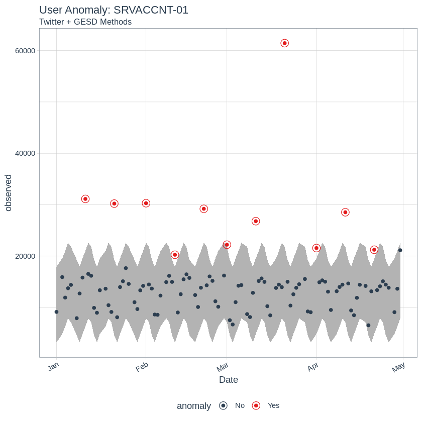
# Filtering dataset for specific User
FilteredAccount = "SRVACCNT-01"

# Ungroup dataset , run Time series decomposition method and plot anomalies
graphUser <- byuser %>%
  filter(AccountName == FilteredAccount) %>% 
  ungroup()%>%
  time_decompose(logoncount, method = "twitter", trend = "3 months") %>%
  anomalize(remainder, method = "gesd") %>%
  time_recompose() %>%
  # Anomaly Visualziation
  plot_anomalies(time_recomposed = TRUE) +
  labs(title = paste0("User Anomaly: ",FilteredAccount), subtitle = "Twitter + GESD Methods")

plot(graphUser)

Registered S3 method overwritten by 'tune':
  method                   from   
  required_pkgs.model_spec parsnip

Converting from tbl_df to tbl_time.
Auto-index message: index = Date

frequency = 6 days

Registered S3 method overwritten by 'quantmod':
  method            from
  as.zoo.data.frame zoo 

median_span = 53 days

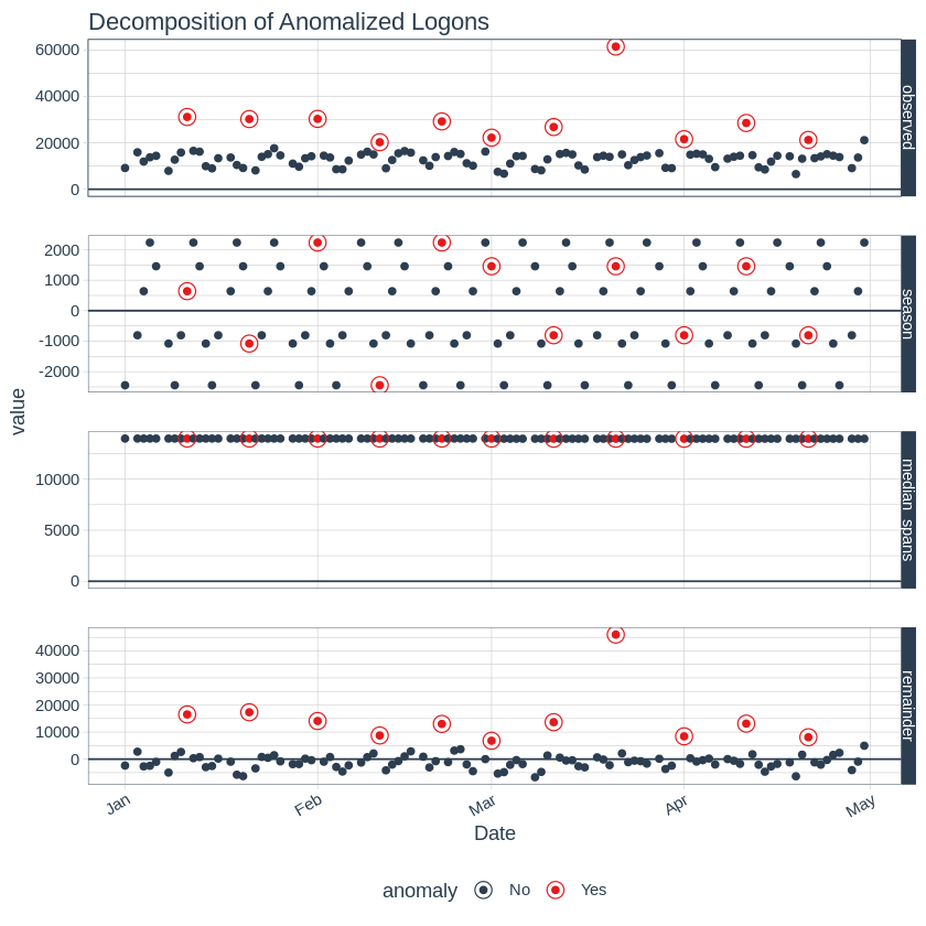
../../_images/1443bd6ed3137a13099aec0bfb9eb0ad8998c11230acd0ccfbf82d58555de759.png

# Plot Time series decompositions components separately
byuser %>%
    filter(AccountName == FilteredAccount) %>% 
    ungroup()%>%
    time_decompose(logoncount, method = "twitter", trend = "3 months") %>%
    anomalize(remainder, method = "gesd") %>%
    plot_anomaly_decomposition() +
    labs(title = "Decomposition of Anomalized Logons")

Converting from tbl_df to tbl_time.
Auto-index message: index = Date

frequency = 6 days

median_span = 53 days

../../_images/4c965a1c0695fae4e287ddc0e2d728a3325e0cafb5b7b488a56dd45c039bf04c.png